40 conditional formatting data labels excel
Conditional Formatting Shapes - Step by step Tutorial 1. Insert a shape on any given worksheet. 2. We choose the oval object: 3. In the Name Box, change the default name to any given name: Why is this important? We store the values and colors that make the object dynamic on the setup sheet. We give every object a specific name and can easily identify them. VBA Conditional Formatting of Charts by Value and Label The category labels (XValues) and values (Values) are put into arrays, also for ease of processing. The code then looks at each point's value and label, to determine which cell has the desired formatting. The rows and columns are looped starting at 2, since the first of each contains an irrelevant label. The looping stops one count before the end.
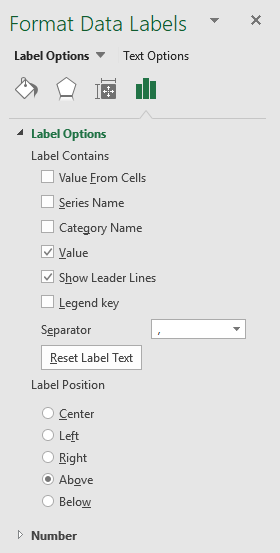
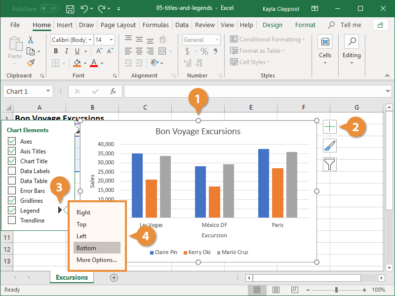
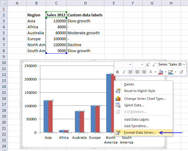
Change the format of data labels in a chart To get there, after adding your data labels, select the data label to format, and then click Chart Elements > Data Labels > More Options. To go to the appropriate area, click one of the four icons ( Fill & Line, Effects, Size & Properties ( Layout & Properties in Outlook or Word), or Label Options) shown here.

Conditional formatting data labels excel
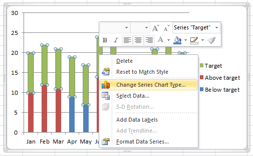
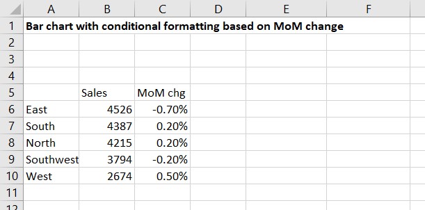
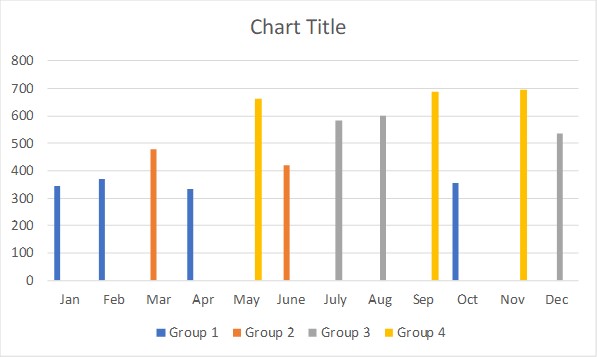
Data Bars in Excel (Examples) | How to Add Data Bars in Excel? - EDUCBA Data Bars in Excel is the combination of Data and Bar Chart inside the cell, which shows the percentage of selected data or where the selected value rests on the bars inside the cell. Data bar can be accessed from the Home menu ribbon’s Conditional formatting option’ drop-down list. If we go there, we will be able to see Gradient Fill and Sold Fill Data bar. Whereas gradient … How to Create Excel Charts (Column or Bar) with Conditional Formatting ... Conditional formatting is the practice of assigning custom formatting to Excel cells—color, font, etc.—based on the specified criteria (conditions). The feature helps in analyzing data, finding statistically significant values, and identifying patterns within a given dataset. Excel bar chart with conditional formatting based on MoM change Click on any bar and press Ctrl+1 to make the Format Data Series task pane appear if it is not already showing. In the Series Options section, set the Gap Width to 50% to give the bars more presence and set the Series Overlap to 100%. Use the chart skittle (the "+" sign to the right of the chart) to remove the legend and gridlines.
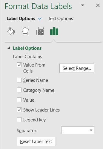
Conditional formatting data labels excel. Use conditional formatting to highlight information Conditional formatting can help make patterns and trends in your data more apparent. To use it, you create rules that determine the format of cells based on their values, such as the following monthly temperature data with cell colors tied to cell values. Excel Data Analysis - Conditional Formatting - tutorialspoint.com Follow the steps to conditionally format cells − Select the range to be conditionally formatted. Click Conditional Formatting in the Styles group under Home tab. Click Highlight Cells Rules from the drop-down menu. Click Greater Than and specify >750. Choose green color. Click Less Than and specify < 500. Choose red color. Create Dynamic Chart Data Labels with Slicers - Excel Campus 10.02.2016 · Typically a chart will display data labels based on the underlying source data for the chart. In Excel 2013 a new feature called “Value from Cells” was introduced. This feature allows us to specify the a range that we want to use for the labels. Since our data labels will change between a currency ($) and percentage (%) formats, we need a ... Excel Conditional Number Formatting In Charts - Stack Overflow I am working with Excel 2010 and I want to apply conditional number formatting to value labels in a chart. When I apply the conditional formatting to the cells within the workbook, the conditional formatting works just fine, but when I feed that data to a chart the conditional number formatting is lost on the value labels.
New Conditional Formatting experience in Excel for the web Jan 20, 2022 · This rule type gives you the added flexibility of formatting a range based on the result of a function or evaluate data in cells outside the selected range. Formula rule type . More coming soon to Conditional Formatting in Excel for the web: Reorder rules with drag & drop ; Change the range the rule refers to in the rule manager ; Custom formatting How to do conditional formatting of a label in Excel VBA Function ConditionalFormatNumber (n As Double) As String If n > 1000000 Then ConditionalFormatNumber = Format (n / 1000000, "$#,##0.00,,""M""") ElseIf n > 1000 Then ConditionalFormatNumber = Format (n / 1000, "$#,##0.00, ""K""") Else ConditionalFormatNumber = Format (n, "$#,##0.0") End If End Function Share Improve this answer Follow A Quick Guide to Conditional Formatting in Excel - HubSpot 1. First, select column B. 2. Navigate to the header toolbar and select Conditional Formatting. When the Conditional Formatting drop-down menu appears, select Highlight Cells Rules, then Equal To. 3. In the New Formatting dialog box, select Cell Value and Equal To. Conditional Formatting in Excel - Step by Step Examples - WallStreetMojo The steps to highlight duplicates in the given range are listed as follows: Step 1: From the "conditional formatting" drop-down in the Home tab, select "highlight cells rules.". Choose the option "duplicate values," as shown in the following image. Step 2: The "duplicate values" window appears.
Progress Doughnut Chart with Conditional Formatting in Excel Mar 23, 2017 · Great question! The Excel Web App does not support those text box shapes yet. We can use the built-in data labels for the chart instead. The label for the Remainder bar can be deleted by left clicking on the label twice, then pressing the delete key. That just leaves the data label for the actual progress amount. Here is a screenshot. Conditional Formatting to Distinguish Between Labels and Numbers I want to conditionally format each cell, so that the text is yellow, the numbers are blue, and the blank cells are green. I tried by setting up a new rule under conditional formatting, then selecting "use a formula to determine which cells to format", then using some combinations of the if, istext, isnumber, etc. combinations. Please advise. Creating Conditional Data Labels in Excel Charts - YouTube We can make labels appear on our charts that don't have to do with the raw numbers that built the chart - and we can make them show up or not based on whatever conditions we want. In this tutorial,... Conditional formatting chart data labels? - Excel Help Forum The easy way to conditionally format these labels is use two series. Use something like =IF ($E2=1,0,NA ()) for the series that has red labels and =IF (#E2=1,NA (),0) for the series that has unformatted labels. Jon Peltier Register To Reply Similar Threads Conditional Number Formatting Not Working for Chart Value Labels
Dynamic Number Format for Millions and Thousands - PK: An ...
How to create a chart with conditional formatting in Excel? - ExtendOffice Add three columns right to the source data as below screenshot shown: (1) Name the first column as >90, type the formula =IF (B2>90,B2,0) in the first blank cell of this column, and then drag the AutoFill Handle to the whole column;

Creating Pie Chart and Adding/Formatting Data Labels (Excel)
Conditional Formatting with Data Validation - Microsoft Tech Community Select the range in column C that you want to format, for example C2:C100. The first cell in the range (C2 in this example) should be the active cell in the selection. On the Home tab of the ribbon, select Conditional Formatting > New Rule... Select 'Use a formula to determine which cells to format'. Enter the formula

CIS Ch3 Excel Flashcards | Quizlet
Excel tutorial: How to use data bars with conditional formatting In the Conditional Formatting menu, data bars are a main category. There are six presets for data bars with gradient fills, and six presets for data bars with solid fills. Except for the fill, these data bar presets are the same. Excel builds a live preview on the worksheet as we hover over each option.

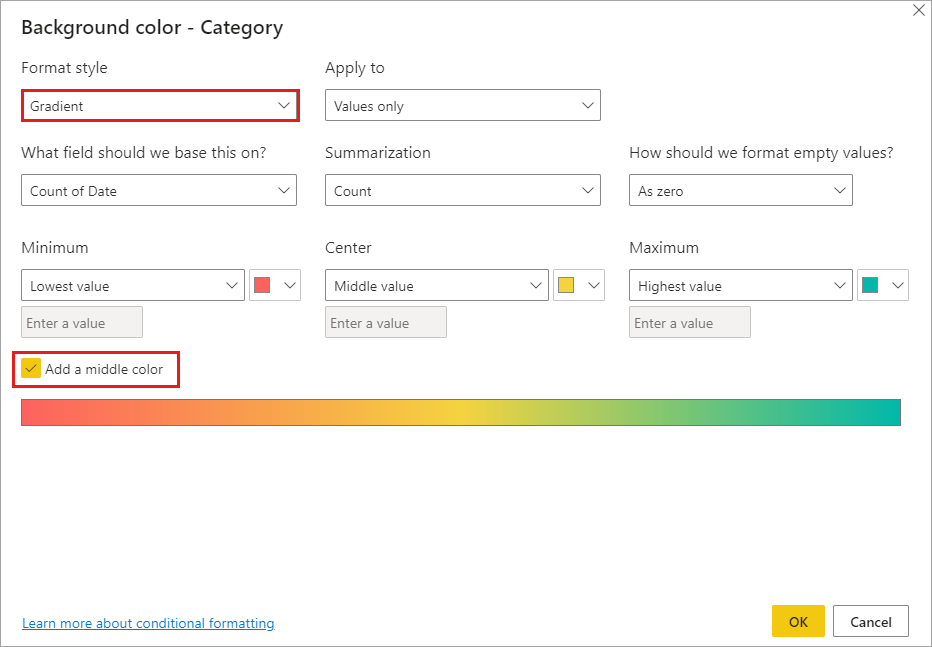
How to improve or conditionally format data labels in Power ...
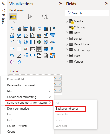
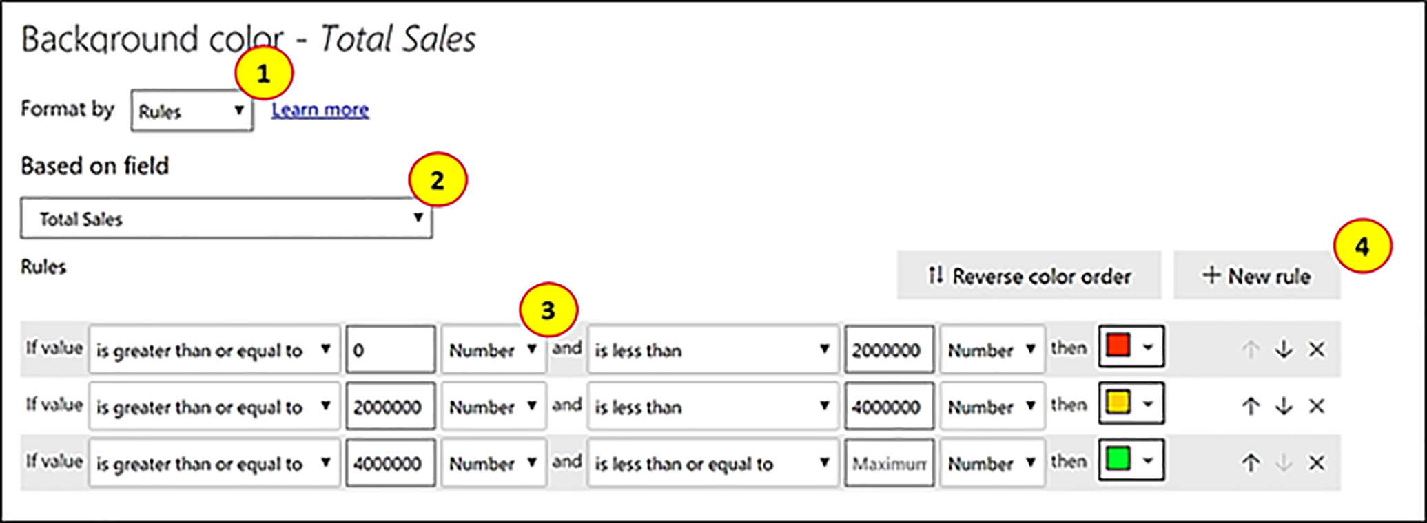
Conditional formatting for Data Labels in Power BI Example-1: Conditional formatting based on Rules. Step-1: Select the visual >go to the format pane>Data Labels. Step-2: Choose measure from "Apply settings to". choose measure. Step-3: Go to Values> Click on fx icon. Step-4: Choose Format Style - Rules and Select measure name. After that add rules condition, see the below given screen shot.

How to Change Excel Chart Data Labels to Custom Values?
How to Change Excel Chart Data Labels to Custom Values? May 05, 2010 · Now, click on any data label. This will select “all” data labels. Now click once again. At this point excel will select only one data label. Go to Formula bar, press = and point to the cell where the data label for that chart data point is defined. Repeat the process for all other data labels, one after another. See the screencast.
How to add and customize chart data labels
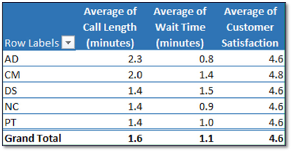
Conditionally Format Values Area Based on Row Labels (LONG) The Row Labels area is one column of job role titles (e.g., Project Manager, System Architect etc.). The Column Labels area includes 6 columns, each of which corresponds to 1 of 6 columns in the source data. These 6 source data columns are personnel utilization values for each of the job roles (e.g., Billable Utilization %, Nonbillable ...
Example: Charts with Data Labels — XlsxWriter Documentation
Excel Icon Sets conditional formatting: inbuilt and custom - Ablebits.com Select the range of cells where you want to apply the icons. Click Conditional Formatting > Icon Sets > More Rules. In the New Formatting Rule dialog box, select the desired icons. From the Type dropdown box, select Percentage, Number of Formula, and type the corresponding values in the Value boxes. Finally, click OK.

Improve your X Y Scatter Chart with custom data labels
How to change chart axis labels' font color and size in Excel? Apply conditional formatting to fill columns in a chart. By default, all data point in one data series are filled with same color. Here, with the Color Chart by Value tool of Kutools for Excel, you can easily apply conditional formatting to a chart, and fill data points with different colors based on point values. Full Feature Free Trial 30-day!
How-to Make Conditional Label Values in an Excel Stacked ...
Easy Conditional Mail Merge Formatting (If...Then...Else): MS … 08.12.2021 · 13. If you want to apply conditional formatting manually, you need to use Ctrl+F9 to add the curly braces and the field codes. Note: Don’t use spaces in your field names. Formatting the Conditional Text in Word Mail Merge. When you perform a merge mail in Microsoft Word, the formatting of an MS Excel data file is lost. You must edit the field ...

Conditional Formatting (Fill Color, Font Color etc...) for ...
Custom Chart Data Labels In Excel With Formulas - How To Excel At Excel Follow the steps below to create the custom data labels. Select the chart label you want to change. In the formula-bar hit = (equals), select the cell reference containing your chart label's data. In this case, the first label is in cell E2. Finally, repeat for all your chart laebls.
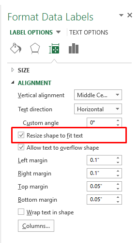
Resize Chart's Data Label Shape To Fit Text|Documentation
How to Apply Conditional Formatting to Pivot Tables - Excel Campus Select a cell in the Values area. The first step is to select a cell in the Values area of the pivot table. If your pivot table has multiple fields in the Values area, select a cell for the field you want to apply the formatting to. 2. Apply Conditional Formatting. You can find the Conditional Formatting menu on the Home tab of the Ribbon.

Color Negative Chart Data Labels in Red with downward arrow
Excel Conditional Formatting not functioning correctly after … Jan 10, 2018 · Everything works fine, formatting changes according to changes in the data! Now I copy a range of sheet A to sheet B using VBA, that works OK. However: in sheet B the conditional formatting of these cells is not working correctly anymore: > cells using 'format only cells that contain' work correct! formatting changes correctly when data changes
Apply conditional table formatting in Power BI - Power BI ...
Conditional Formatting of Excel Charts - Peltier Tech Conditionally Formatted Line Chart. The data for the conditionally formatted bar chart is shown below. The formatting limits are inserted into rows 1 and 2. The header formula in cell C3, which is copied into D3:G3, is. =C1&"

Color Negative Chart Data Labels in Red with downward arrow
Conditional Formatting Using Custom Measure - Power BI 28.09.2020 · Voila! We have given conditional formatting to Day of Week column based on the clothing Category value. I just tried to add a simple legend on the top to represent the color coding. So, this is how one can use a custom color formatting in Power BI by creating a simple measure for it. Hope this article helps everyone out there. - Pragati

Change the format of data labels in a chart
Conditional formatting with formulas (10 examples) | Exceljet You can create a formula-based conditional formatting rule in four easy steps: 1. Select the cells you want to format. 2. Create a conditional formatting rule, and select the Formula option 3. Enter a formula that returns TRUE or FALSE. 4. Set formatting options and save the rule.

Enhance the Card Visual in Power BI with Conditional ...
How to Apply Different Types of Conditional Formatting in Excel How to Apply Data Bars Conditional Formatting in Excel. The third type of conditional formatting in Excel is Data Bars. So this will create bars in our data set representing both the positive and negative values. And to apply this type of conditional formatting in Excel, let's learn the following steps below: 1. Firstly, select the needed ...
Format Chart Numbers as Thousands or Millions — Excel ...
Changing the Color of a Data Label using IF Statement 1) Click on the data labels to highlight all the data labels, 2) Right-Click and select Format Data Labels, 3) Click on Number, 4) Go to the Format Code field *adapt the following to your needs* 5) [green] [>29]#.00; [<30] [Color 53]#.00 Click to expand... Hi Jawnne, I hope you're still lurking about on here.

How to show percentages on three different charts in Excel ...
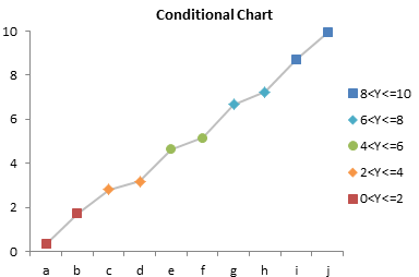
r/excel - Is it possible to conditionally format Data Labels on a ... On a dynamic line chart, where Y-axis is scaled from 0-10 and X-axis is dates, is it possible to conditionally format Data Labels such that the colour of the data labels changes based on the data values that are plotted. For example, when numbers 0-3 are plotted on the dynamic chart above their data label's font colour turns red, and if numbers ...

Conditional formatting by field value in Power BI - Power BI Docs
Conditional Formatting For Blank Cells - EDUCBA Always use limited data to deal with and apply bigger conditional formatting to avoid excel getting freeze. Recommended Articles. This has been a guide to Conditional Formatting for Blank Cells. Here we discuss how to apply Conditional formatting for blank cells along with practical examples and a downloadable excel template. You can also go ...

Apply Custom Data Labels to Charted Points - Peltier Tech
Excel bar chart with conditional formatting based on MoM change Click on any bar and press Ctrl+1 to make the Format Data Series task pane appear if it is not already showing. In the Series Options section, set the Gap Width to 50% to give the bars more presence and set the Series Overlap to 100%. Use the chart skittle (the "+" sign to the right of the chart) to remove the legend and gridlines.
How to Create Excel Charts (Column or Bar) with Conditional ...
How to Create Excel Charts (Column or Bar) with Conditional Formatting ... Conditional formatting is the practice of assigning custom formatting to Excel cells—color, font, etc.—based on the specified criteria (conditions). The feature helps in analyzing data, finding statistically significant values, and identifying patterns within a given dataset.
Power BI Conditional Formatting | Burningsuit
Data Bars in Excel (Examples) | How to Add Data Bars in Excel? - EDUCBA Data Bars in Excel is the combination of Data and Bar Chart inside the cell, which shows the percentage of selected data or where the selected value rests on the bars inside the cell. Data bar can be accessed from the Home menu ribbon’s Conditional formatting option’ drop-down list. If we go there, we will be able to see Gradient Fill and Sold Fill Data bar. Whereas gradient …
Create charts with conditional formatting – User Friendly

How-to Make Conditional Data Labels for an Excel Dashboard

Solved: Conditional Formatting of Bar Chart - Microsoft Power ...
How to Edit a Legend in Excel | CustomGuide

Highlight Max & Min Values in an Excel Line Chart - Xelplus ...
Conditional Formatting of Excel Charts - Peltier Tech
Excel bar chart with conditional formatting based on MoM ...
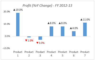
Color Negative Chart Data Labels in Red with downward arrow
Excel bar chart with conditional formatting based on MoM ...

Is it possible to conditionally format Data Labels on a ...

Highlight Max & Min Values in an Excel Line Chart - Xelplus ...
Excel tutorial: How to use data labels

Dynamically Label Excel Chart Series Lines • My Online ...
Apply conditional table formatting in Power BI - Power BI ...
Excel - Beyond the Basics Part Two: Using Conditional ...
Custom data labels in a chart
Conditional Formatting of Excel Charts - Peltier Tech
Conditional formatting for Excel column charts | Think ...
Post a Comment for "40 conditional formatting data labels excel"